Navigation :

Introduction to RAD-Seq

Note: Currently, this tutorial is written to be performed on the mozzie server. In the future, this will be expanded so it can be done on any linux server.

This tutorial goes through the steps of setting up a project directory, demultiplexing RAD-Seq data, aligning RAD-seq samples to a reference genome, building the loci catalogue and calling SNPs with Stacks, and generating a PCA plot of the SNP data.

Pre-requisites

Before beginning this tutorial, you should be familiar with RAD-seq for SNP discovery. If you’re not familiar with RAD-seq, we recommend you read this review paper to help you get started.

This tutorial also assumes you’re familiar with Unix and running commands on the command line interface. If you’re using a shared cluster, you should also be familiar with running jobs through SLURM.

The last section also assumes some basic knowledge of R.

Learning objectives

Understand the nature of RAD-seq sequencing data
Process ddRAD data using the Stacks reference-based workflow
Be able to calculate some statistics and generate a PCA plot using the SNP results

The data

The data this tutorial uses is from Aedes Aegypti mosquitos collected from Indonesia and Malaysia. The samples were prepared following a protocol adapted from the methods described here. The restriction enzymes used for the double digest were nlaIII and mluCI.

To save time, we’ll be using a subset of the full data in this tutorial. Only reads belonging to Aedes Aegypti Chr1:1-1000000 have been included in the sequencing data.

The size of the tutorial data is around 500 MB. In real situations, you would expect libraries to be in the order of 10s of gigabytes, and have multiple libraries in a project.

Setup the project directory

Let’s begin by setting up a directory for your project. Good project organisation will make your life easier in the long run, so spend some time at the outset to do it properly. A few months after your initial analysis, you may not remember what you did or what your files contain. Detailed documentation and a sensible directory structure can help with this.

Go to the directory where you wish to store this project, and create a new directory for this tutorial. An example project name could be rad_seq_tutorial.

cd /path/to/sensible/project/directory
mkdir rad_seq_tutorial
cd rad_seq_tutorial

# Store the tutorial path in a variable so we can refer to it later
TUTORIAL_DIR=$(pwd)

In this directory, we’ll create some new directories where we’ll store our data and results.

mkdir raw_data demuxed_seq results scripts software

We’ll also create a few sub-directories in results where we’ll store output from different programs that we’ll run. These will be stored in results_2020-02-01 (change the date to your current date). When performing bioinformatics, it’s not unusual to have to re-run analyses again sometime down the track (e.g. the addition of a new sequencing library, changing of parameters for tools, fixing mistakes). Including the date in the directory name is an easy way to identify different sets of analyses in the future.

cd results
mkdir results_2020-02-01
cd results_2020-02-01
mkdir alignments gstacks populations

Lastly, create a README.txt text file with a brief description of what the project directory is about using your favourite text editor. For example:

# RAD-seq Tutorial

This directory contains analysis of RAD-seq data from Indonesia and Malaysia 
from the Intro to RAD-Seq tutorial.

Your project directory should look something like this:

rad_seq_tutorial/
├── demuxed_seq/
├── raw_data/
├── results/
│   ├── results_2020-02-01/
│   │   ├── alignments/
│   │   ├── gstacks/
│   │   └── populations/
├── scripts/
├── software/
└── README.txt

Get the data

If you’re using the mozzie server, copy the files in /mnt/galaxy/shared/tutorial_data/rad_seq_workshop/ into the raw_data directory of your tutorial project directory.

cd $TUTORIAL_DIR
cd raw_data
cp -r /mnt/galaxy/shared/tutorial_data/rad_seq_workshop/* .

Note that our library data is stored in another sub-directory, tute_library. It’s common to have multiple libraries for a single project, therefore a good idea to have a separate sub-directories for each of your libraries.

In the library directory, the paired end sequencing data is in the two FASTQ files:

tute_library_R1.fastq.gz corresponds to the forward reads from a PE library
tute_library_R2.fastq.gz corresponds to the reverse reads from a PE library

Also included is:

barcodes.txt: the barcode file that will be used to separate individual samples from the FASTQ file

There are also two files called popmap_01.txt and popmap_02.txt that we’ll discuss later.

Your raw data directory should now look like this:

raw_data/
├── tute_library/
│   ├── barcodes.txt
│   ├── tute_library_R1.fastq.gz
│   └── tute_library_R2.fastq.gz
├── popmap_01.txt
└── popmap_02.txt

Demultiplexing

Examine the data

Multiple samples are sequenced in a single RAD-seq library. Each sample has a unique combination of barcodes that we can use to separate which reads belong to each sample. The program that we’ll use, process_radtags, requires this information to be in a specific form.

Navigate to the raw_data/tute_library directory. Take a look at the barcodes.txt file to see an example of a barcode file.

cat barcodes.txt

CTAGTC	GTACTG	indonesia_01
AGCTGA	GTACTG	indonesia_02
TCGACT	GTACTG	indonesia_03
ATGCTA	GTACTG	indonesia_04
GCATAG	GTACTG	indonesia_05
TGCACA	CATGAC	malaysia_01
CATGTG	CATGAC	malaysia_02
GTACAC	TGCAGT	malaysia_03
ACGTGT	TGCAGT	malaysia_04
AGCTCT	TGCAGT	malaysia_05
GATCTC	TGCAGT	unknown_01
AGCTGA	ACGTCA	unknown_02

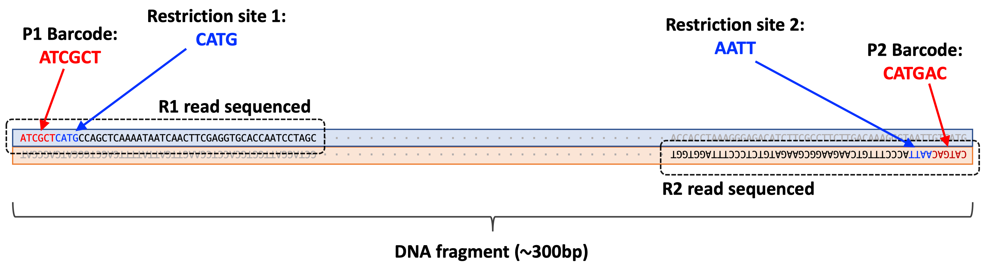
The barcode file is a tab-separated file where the first column corresponds to the p1 barcode (the barcode that will be found at the beginning of the read), the second column corresponds to the p2 barcode (the barcode that will be found a the end of the read), and the third column represents the sample name.

From this file, we can see there are 12 samples we’d like to demultiplex from the library: five samples from Indonesia, five from Malaysia, and two samples that have not been labelled with their location of origin.

Let’s now have a look at the raw FASTQ data. If you’re unfamiliar with the FASTQ format, you can read up on it here.

Use less to view the R1 reads (i.e. the forward reads of this library):

less tute_library_R1.fastq.gz
# press 'q' to quit when you're done

Look at the first read of the file which makes up the first four lines:

@SN7001291:345:HFKWVBCXX:2:1101:1829:1987 1:N:0:2
ATCGCTCATGCCAGCTCAAAATAATCAACTTCGAGGTGCACCAATCCTAGCGCTATCAGACCTCCCTCGCTATGAGACGGCTGCGCATTTTCATTCCCTTG
+
GGGGGIIIIIIIIIIIIIIIIIIIIIIIIIIIIGIIIIIIIIIIIIIIIGGGGIIIIIIIGIIIIIIIIIIIIIIIIIIIIIGIGIGGGIIIIIIIIIGGG

The first line contains the read identifier. Each identifier begins with an @ character and is unique.
The second line contains the nucleotide sequence of the read.
The third line is a separator line and contains a + character.
The fourth line contains the PHRED quality score (i.e. a measurement of base confidence) for each of the bases in the nucleotide sequence.

Let’s look at the second line (i.e. the sequence) more closely:

ATCGCTCATGCCAGCTCAAAATAATCAACTTCGAGGTGCACCAATCCTAGCGCTATCAGACCTCCCTCGCTATGAGACGGCTGCGCATTTTCATTCCCTTG

The first six bases (e.g. ATCGCT) of each read in this file correspond to the p1 barcode sequence. The next four bases are CATG which corresponds to the restriction site where nlaIII cleaves.

5'-   C A T G | -3'
3'- | G T A C   -5'

All reads in the R1 file should have this restriction site sequence immediately following the barcode sequence.

Now, look at the R2 file (i.e. the reverse reads):

less tute_library_R2.fastq.gz
# press 'q' to quit when you're done

The first read in this file is

@SN7001291:345:HFKWVBCXX:2:1101:1829:1987 2:N:0:2
CATGACAATTACCCTTTGTCAAGAAGGCGAAGATGTCTCCCTTTAGGTGGTAAGTCAACTTACCAGAAAGAAGTTGAGCAATGTGGAAAAATCCACCATTC
+
GGIGGIGGIGIGIGGIIIIIIIIIIGIIGIGIIIGIIGGGIIGGGGGAGGGIIIIIIIIIIGIIIIIIIIIGIIIIIIIIIIIGIIIIIIIIIIIIGGGGG

Like the R1 file, the first six bases (CATGAC) correspond to the p2 barcode sequence. Since the first read of the R1 file and the first read of the R2 file are mate pairs (i.e. they were sequenced from the same DNA fragment), we can use both the p1 and p2 barcodes to determine what sample the sequence belongs to.

The next four bases are AATT which corresponds to the restriction site were mluCI cleaves.

5'- | A A T T   -3'
3'-   T T A A | -5'

These two reads are both sequenced from the same DNA fragment.

Question:
For a specific set of paired-end reads, the p1 barcode is observed to be ATGCTA and the p2 barcode is observed to be GTACTG. What sample does the read belong to?
Answer:
indonesia_04

Run process_radtags

The Stacks suite has a program called process_radtags that demultiplexes RAD-seq data. We’ll run it on our tutorial data and provide it the barcode file like so:

cd $TUTORIAL_DIR

process_radtags \
    -1 raw_data/tute_library/tute_library_R1.fastq.gz \
    -2 raw_data/tute_library/tute_library_R2.fastq.gz \
    -o demuxed_seq \
    -b raw_data/tute_library/barcodes.txt \
    --renz_1 nlaIII \
    --renz_2 mluCI \
    --paired \
    -i gzfastq \
    --inline_inline \
    -c -q -r -t 80 -s 20

Generally, if you’re running commands on a shared server, you should be using SLURM to submit your jobs. However, this tutorial data only takes a few seconds to process, so if you’re using the mozzie server, you can just run it on the master node without SLURM. With real data, jobs can take hours to run, so make sure you don’t run large jobs on the master node.

process_radtags produces four files for each sample. For example, for indonesia_01:

indonesia_01.1.fq.gz: contains R1 (forward) reads belonging to the sample
indonesia_01.2.fq.gz: contains R2 (reverse) reads belonging to the sample
indonesia_01.rem.1.fq.gz: contains orphaned R1 reads that don’t have a matching R2 read
indonesia_01.rem.2.fq.gz: contains orphaned R2 reads that don’t have a matching R1 read

Reads can be orphaned when the mate pair’s read restriction enzyme site doesn’t match or the read is dropped due to low quality.

Question:
Have a look at the log file in process_radtags. How many reads matched the barcode for the indonesia_01 sample? After filtering those without a matching restriction site and low quality, how many reads have been retained for indonesia_01?
Answer:
258052 total sequences matched indonesia_01. 229479 were retained after removing reads with restriction site not matching (23282) and of low quality (5291).

Question:
In the process_radtags command you ran, what does the option -t 80 and -s 20 do? (Hint: check the manual)
Answer:
The “-t 80” option truncates the read to a final length of 80 bp. The “-s 20” option tells the program to discard the read due to low quality if the average quality score drops below 20 in a sliding window (whose size is set by the “-w” option and has a default of 0.15).

In this tutorial, we have trimmed reads to 80 bp, as our sequence reads are 100 bp. If you’re using new sequencing data, your reads may be 150 bp reads, and you should trim these to a longer length such as 130 bp or 140 bp. If you don’t know what length your sequence reads are, make sure you find out before progressing further in this analysis. One method to do this is to run FastQC on your raw FASTQ files.

Alignment

The reference genome

Next we’ll align the demultiplexed reads to the reference Aedes Aegypti reference genome using bowtie2. First, have a look at the reference assembly FASTA file. On the mozzie server:

cd /mnt/galaxy/shared/genomes/GCF_002204515.2_AaegL5.0
less GCF_002204515.2_AaegL5.0_genomic.fna
# press 'q' to quit when you're done

This large file contains the 1.9 gigabases that make up the Aedes Aegypti genome. Most of the bases have been assembled into three chromosomes: NC_035107.1 (chr1), NC_035108.1 (chr2), and NC_035109.1 (chr3). Since the assembly is imperfect, there are also thousands of smaller scaffolds that have yet to be placed to a chromosome.

If you’re working on the mozzie server, the genome has already been indexed and is ready to be used for alignment with bowtie2. If you’re working on another server, you’ll need to download the genomic FASTA file for GenBank assembly GCF_002204515.2 yourself. You’ll also need to build a Bowtie index for the reference genome using bowtie2-build.

Bowtie2

Alignment is the process of mapping reads from your FASTQ files to a location on the reference genome. Bowtie2 is a commonly used aligner that can quickly align short reads to a reference. We’ll now align the demultiplexed reads to the Aegypti reference genome we viewed earlier. For indonesia_01:

cd $TUTORIAL_DIR/results/results_2020-02-01

bowtie2 \
  -p 2 \
  -x /mnt/galaxy/shared/genomes/GCF_002204515.2_AaegL5.0/GCF_002204515.2_AaegL5.0_genomic \
  --very-sensitive \
  -1 ../../demuxed_seq/indonesia_01.1.fq.gz \
  -2 ../../demuxed_seq/indonesia_01.2.fq.gz \
  2> alignments/indonesia_01.bt2.log \
  | samtools view -bS \
  | samtools sort -o alignments/indonesia_01.bam

We’ve chosen the --very-sensitive preset option which is through in trying to align reads to the reference genome, but takes a longer time than other presets. The SAM output from bowtie2 is piped into samtools to convert it to BAM, and then piped again to sort the BAM file. If you’re unfamiliar with the SAM/BAM format, you can read up on it here.

Take a look at the BAM file:

samtools view alignments/indonesia_01.bam | less
# press q to quit when you're done

If you want to have a more in-depth look at the options that bowtie2 has, you can view the help message with the -h flag:

bowtie2 -h

or have a look at the bowtie2 manual.

We can also write a loop to process all samples sequentially. For example, the code below uses the barcode file’s to extract the sample names in the library, and then runs bowtie2 on the sample’s demultiplexed FASTQ file.

while read line; do
    sample=$(echo $line | cut -d " " -f 3)
    echo Aligning sample: $sample
    bowtie2 \
        -p 2 \
        -x /mnt/galaxy/shared/genomes/GCF_002204515.2_AaegL5.0/GCF_002204515.2_AaegL5.0_genomic \
        --very-sensitive \
        -1 ../../demuxed_seq/${sample}.1.fq.gz \
        -2 ../../demuxed_seq/${sample}.2.fq.gz \
        2> alignments/${sample}.bt2.log \
        | samtools view -bS \
        | samtools sort -o alignments/${sample}.bam
done < ../../raw_data/tute_library/barcodes.txt

Question:
Take a look at the log file malaysia_02.bt2.log. What is the overall alignment rate for the sample? Given what you know about this tutorial data, why might this alignment rate be higher than normal?
Answer:
The observed overall alignment rate of this sample is 93.84%. This alignment rate is not representative of a real RAD-seq experiment because the tutorial data is made up of reads that were selected because they were known to align to a defined part of this genome. If we were working with the full set of data, the alignment rate would be reduced.

Stacks

Stacks is a suite of software tools that can processes RAD-seq data, call SNPs, and calculate some popgen statistics. In reference-based RAD-seq analysis, we’ll be using the programs gstacks and populations.

Run gstacks

The next step is to build a catalogue of RAD-tags using gstacks. You can read more about the program and its options here.

There are two valid ways you can define which BAM files you input into gstacks: using a popmap file or listing each bam file in the command. We’ll be using the latter. Here we’ll use the -M argument to give gstacks a popmap file and the -I argument to give it our alignments directory.

The popmap file is a simple tab-delimited file that defines what population each sample is from. The populations program that we’ll run immediately after gstacks can use this information to calculate common population genetics statistics such as FST and nucleotide diversity.

In some cases, you won’t be interested in the statistics calculated by populations (since you’ll be doing your own analyses downstream). If this is the case, you can just define all samples as belonging in the same group. Have a look at the popmap file included in the raw_data directory:

cd $TUTORIAL_DIR/raw_data/
cat popmap_01.txt

In this directory, there’s also another popmap file called popmap_02.txt. You can use this popmap file if you want to define groups in downstream Stacks analysis.

Question:
Have a look at the popmap_02.txt file. How many unique populations are there?
Answer:
There are three unique populations in the file: “indonesia”, “malaysia”, and “unknown”.

Now go back to the results directory and run gstacks to create the catalogue. We’ll use the popmap_01.txt file here, but note that gstacks doesn’t use the population information, only populations does.

cd $TUTORIAL_DIR/results/results_2020-02-01
gstacks \
    -I alignments \
    -M ../../raw_data/popmap_01.txt \
    -O gstacks \
    --min-mapq 20 \
    -t 4

Have a look at the catalog.fa.gz output from gstacks using less.

catalog.fa.gz is a FASTA file that contains the RAD tags that have been detected in the given RAD-seq samples. The header of each sequence contains the position of where the RAD-tag is in the reference genome (e.g. pos=CM008043.1:9352:-) and the number of samples the RAD-tag was found (e.g. NS=1).

catalog.calls is a binary file that contains the genotyping data that populations will use for calling SNPs.

Run populations

Populations can do a number of calculations and statistical tests, but for this tutorial, we’ll only be using it to output a VCF file of our SNP calls. You can read up on populations here.

When we run populations, we’ll be writing to a sub-directory in the populations results directory. It can be useful to have multiple directories for populations as re-running it with different parameters, samples, etc. is common.

Run populations requiring no missing data for any SNPs:

mkdir populations/pop_01
populations \
    -P gstacks \
    -M ../../raw_data/popmap_01.txt \
    -O populations/pop_01 \
    -t 1 \
    -p 1 \
    -r 1 \
    --write_single_snp \
    --vcf

Have a look at the VCF file. If you’re not familiar with the VCF format, you can read up on it here.

Question:
Approximately many SNPs are there in the VCF file?
Answer:
There are 987 SNPs in the VCF file.

Question:
For the first SNP in the VCF file (chromosome NC_035107.1, position 119501), what is the genotype call for indonesia_01? What nucleotide bases would be observed?
Answer:
For indonesia_01, the GT field is “0/1” which means the sample is heterozygous at that position. Since the REF base is C and the ALT base is A, the genotype would be C/A.

Re-run populations in a new directory (pop_02) using less stringent parameters. For this example, we’ll use the popmap_02.txt file to define populations and require SNPs to be called in at least 80% of individuals (-r 0.8) in at least two of the three populations (-p 2). We’ll also include the --fstats flag to enable SNP-based F-statistics.

mkdir populations/pop_02
populations \
    -P gstacks \
    -M ../../raw_data/popmap_02.txt \
    -O populations/pop_02 \
    -t 1 \
    -p 2 \
    -r 0.8 \
    --write-single-snp \
    --vcf \
    --fstats

Since we defined populations and use the --fstats option, we now are given pairwise estimates of FST in our output. Go to the output directory and view some of these files. The files beginning with populations.fst_* contain the SNP-level measures of FST between two populations and populations.fst_summary.tsv contains the pairwise FSTs for the populations.

Additionally, with our less stringent parameters, the new VCF file now has more than twice the number of SNPs included, but some samples have missing genotype calls (i.e. ./.).

Question:
What does the --write-single-snp option do in populations? Why might you want to use this option when you run populations? (Hint: look at the help page or manual)
Answer:
The “--write-single-snp” restricts analysis to only use the first SNP on the RAD tag. Often you want your SNPs to be independent observations (i.e. not under linkage disequilibrium). Using the “--write-single-snp” or “--write-random-snp” flag removes SNPs which are located on the same RAD tag, and therefore very close together in the genome.

Downstream analysis

Generally, the VCF files from populations will form the basis of your downstream analysis of population genetics.

Here, we’ll go through a toy example of using the SNP data to produce a PCA plot and identifying which populations the two unknown samples belong to, but for serious popgen analysis, you’ll need to turn to software packages like adegenet, vegan, and pegas.

We’ll first convert the VCF file into a “012” matrix using VCFtools. This format represents homozygous REF calls as “0”, heterozygous calls as “1” and homozygous ALT calls as “2”.

# Go to the pop_01 directory of populations
cd $TUTORIAL_DIR/results/results_2020-02-01/populations/pop_01

vcftools \
    --vcf populations.snps.vcf \
    --012 \
    --out populations.snps

Have a look at the output files produced by VCFtools.

The next step is to load the files into R. If you’re on the mozzie server, you can just use the RStudio server provided. If you’re not using the mozzie server, download the populations.snps.012 and populations.snps.012.indv files to your local computer.

In R, this code generates a simple PCA plot:

# Load libraries
library(ggplot2)
library(stringr)

# Load 012 files (change the paths)
gt_matrix <- read.table(file="/path/to/rad_seq_tutorial/results/results_2020-02-01/populations/pop_01/populations.snps.012",
                        row.names = 1, header=FALSE)
sample_names <- read.table(file="/path/to/rad_seq_tutorial/results/results_2020-02-01/populations/pop_01/populations.snps.012.indv",
                           header=FALSE)

# View the first bit of the genotype matrix
gt_matrix[1:5,1:5]

# Create a dataframe containing sample info
sample_info <- data.frame(
  sample_id=sample_names[,1],
  group=str_remove(sample_names[,1], "_\\d\\d$"),
  stringsAsFactors=FALSE)
sample_info

# PCA plot
pca <- prcomp(gt_matrix)$x[,1:4]
pca <- cbind(pca, sample_info)
ggplot(pca, aes(x=PC1, y=PC2, color=group)) +
  geom_point()

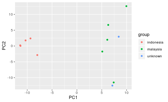
Question:
There are two samples from unknown origin. After looking at the PCA plot, what country do you think they originate from?
Answer:
The two unknown samples both cluster more closely to the Malaysian samples, so it is likely they are from Malaysia.